




Abstract
Background:
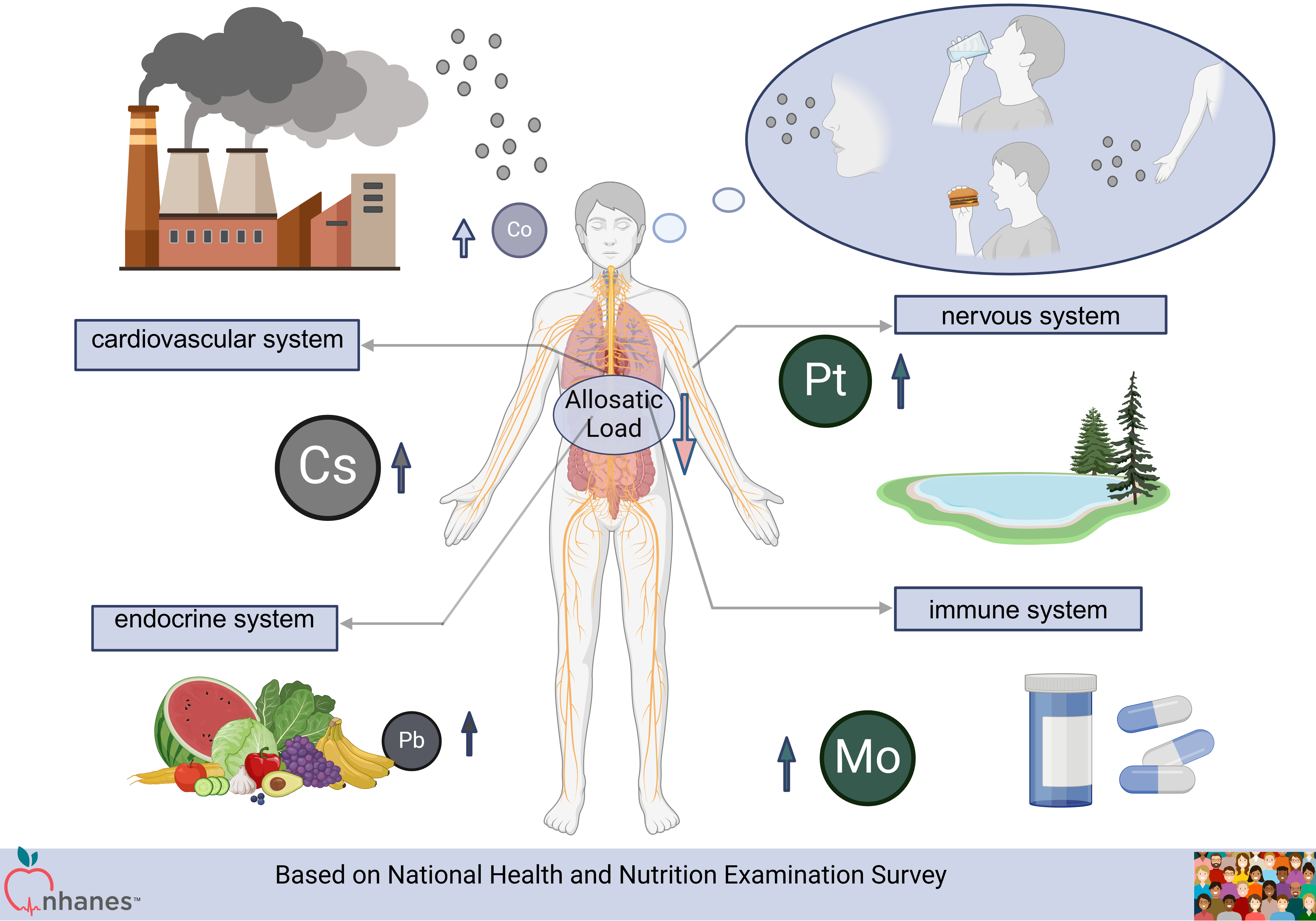
Allostatic load, defined as the cumulative strain resulting from the chronic stress
response, is associated with adverse health outcomes. Heavy metals, prevalent in various
environmental pollutants, exert cumulative effects on the human body through exposure
via water or food sources. However, the relationship between heavy metals and allostatic
load remains poorly understood. The aim of this study is to examine the association
between urinary metal concentrations and allostatic load.
MethodsThis study analyzed data from 4,231 adult participants in the National Health and Nutrition Examination Survey (NHANES) conducted between 2005 and 2010. We employed linear regression analysis, Bayesian kernel machine regression (BKMR), weighted quantile sum (WQS), and quantile g-computation (qgcomp) to investigate the associations between twelve urinary metals and allostatic load. Additionally, we developed K-nearest neighbors (KNN), random forest (RF), and XGBoost models to predict allostatic load scores (ALS).
Results:Linear regression analysis indicated that the combined effects of the twelve urinary metals were negatively correlated with allostatic load. WQS, qgcomp, and BKMR analyses identified cesium (Cs), molybdenum (Mo), lead (Pb), platinum (Pt), and cobalt (Co) as the primary influencing factors (all p-values < 0.05). Furthermore, when predicting ALS based on heavy metal exposure, the random forest model outperformed the other machine learning algorithms, with a root mean square error (RMSE) of 2.377428, compared to 2.501523 for KNN and 2.377733 for XGBoost.
Conclusion:Our findings indicate that urinary metal concentrations are negatively associated with allostatic load, with Cs, Mo, Pt, Pb, and Co showing the most significant negative correlations. Further research is necessary to explore the causal relationships and underlying mechanisms. Additionally, our analysis demonstrated that the random forest model was the most effective for ALS prediction.
Keywords:Electromagnetic radiation; Offspring; Nerve; Reproductive
system;
Introduction
The concept of allostatic load which McEwen and Stellar[1] proposed in an effort to elucidate the process in which various body systems adapt and fluctuate to meet the demands of stress reflects the biological burden of chronic exposure to the downstream effects of various stress-response pathways arising from repeated environmental and physiological challenges[2] . Previous studies have shown that individuals with high AL compared with those with low AL had an increased mortality risk of 22% for all-cause and 31% for CVD mortality[3] . Prior reports also suggested that increased AL disrupt the nervous system and the stress response axis resulting in the disturbance of immune, cardiovascular, metabolic, and neuroendocrine systems, and further increasing cancer risk [4] [2,5] ,even death [6] . In addition to some known potential risk factors such as health-damaging behaviors, there may be some risk factors. Identifying potential risk factors for allostatic load is important for understanding how these factors are associated with physiology as well as health and aging outcomes. Allostatic load can be quantified by the allostatic load score, an established measure of the cardiovascular, metabolic, and immune ramifications of stress, which was found to be a good predictor of mortality and decline in physical functioning [7] [8] [9] .
Heavy metals are commonly defined as metallic elements with a density of ≥ 5 g/cm³. Lead (Pb), cadmium (Cd), mercury (Hg), selenium (Se), and manganese (Mn) are widely distributed environmental pollutants. Humans are commonly exposed to heavy metals through various sources such as air pollution, domestic effluents, cosmetic products, and food consumption[10] . Growing evidence indicates that heavy metals exert toxicity to individuals by interfering with immune homeostasis and promoting inflammation [4] .We have known that physical stressors such as traumatic, infectious, and inflammatory exposures, as well as psychosocial stressors may each lead to frequent activation of allostatic systems, which may lead to high allostatic load [11] .We surmise that exposure to mixture of heavy metals can be associated to high allostatic load.
The study of heavy metal exposure and allostatic load will help us to think about the multilevel physiological regulation and pathological response. At the level of antioxidant and detoxification systems, heavy metals (such as Hg and Cd) can alleviate oxidative damage by inducing the expression of metallothionein, glutathione (GSH) and antioxidant enzymes (catalase, superoxide dismutase) [12] . For example, the lungs of rats exposed to mercury vapor locally adapt by upregulating metallothionein and glutathione, while the kidneys and brain are more vulnerable due to metabolic differences[12] . Cadmium exposure alleviates kidney injury by activating autophagy related genes (Beclin1, LC3), but inhibits the expression of bone formation genes (Osterix, RUNX2), which may lead to osteoporosis risk[13] . However, there are significant differences in detoxification thresholds among different organs, suggesting the need to establish organ-specific exposure limits.
At the same time, long-term low-dose exposure can trigger immune regulatory imbalance, which is manifested by the activation of pro-inflammatory factors (TNF-α, IL-2) pathways and the coexistence of immunosuppressive mechanisms, and this dual effect may increase susceptibility to infection or the risk of autoimmune diseases[13] .
Meanwhile, the study of the relationship between heavy metals and adaptive load has far-reaching significance for the multidimensional strategy of public health intervention, such as the establishment of a biomarker early warning system integrating antioxidant indicators (catalase activity), detoxifying proteins (metallothiosin) and genetic damage markers, [12,14] and further combining regional pollution characteristics to develop differentiated management policies.
In this study, we employed data from the National Health and Nutrition Health and Nutrition Examination Survey (NHANES) in the United States to assess the relationship between allostatic load and the levels of 12 metals—barium (Ba), Beryllium(Be),cadmium (Cd), cobalt (Co), cesium (Cs), molybdenum (Mo), lead (Pb), antimony (Sb), thallium (Tl),platinum(Pt), tungsten (W), and uranium (U)—and their mixture in urine. We employed several statistical models, including multiple logistic regression, weighted quantile sum regression (WQS), Bayesian kernel machine regression (BKMR), to conduct our evaluation. Our findings yield epidemiological evidence for future research on the relationship between combined heavy metals exposure and allostatic load. And we found three ML models that could be used to identify ALS by heavy metals' exposure and then compared the performance characteristics of our models.
Methods
Study population
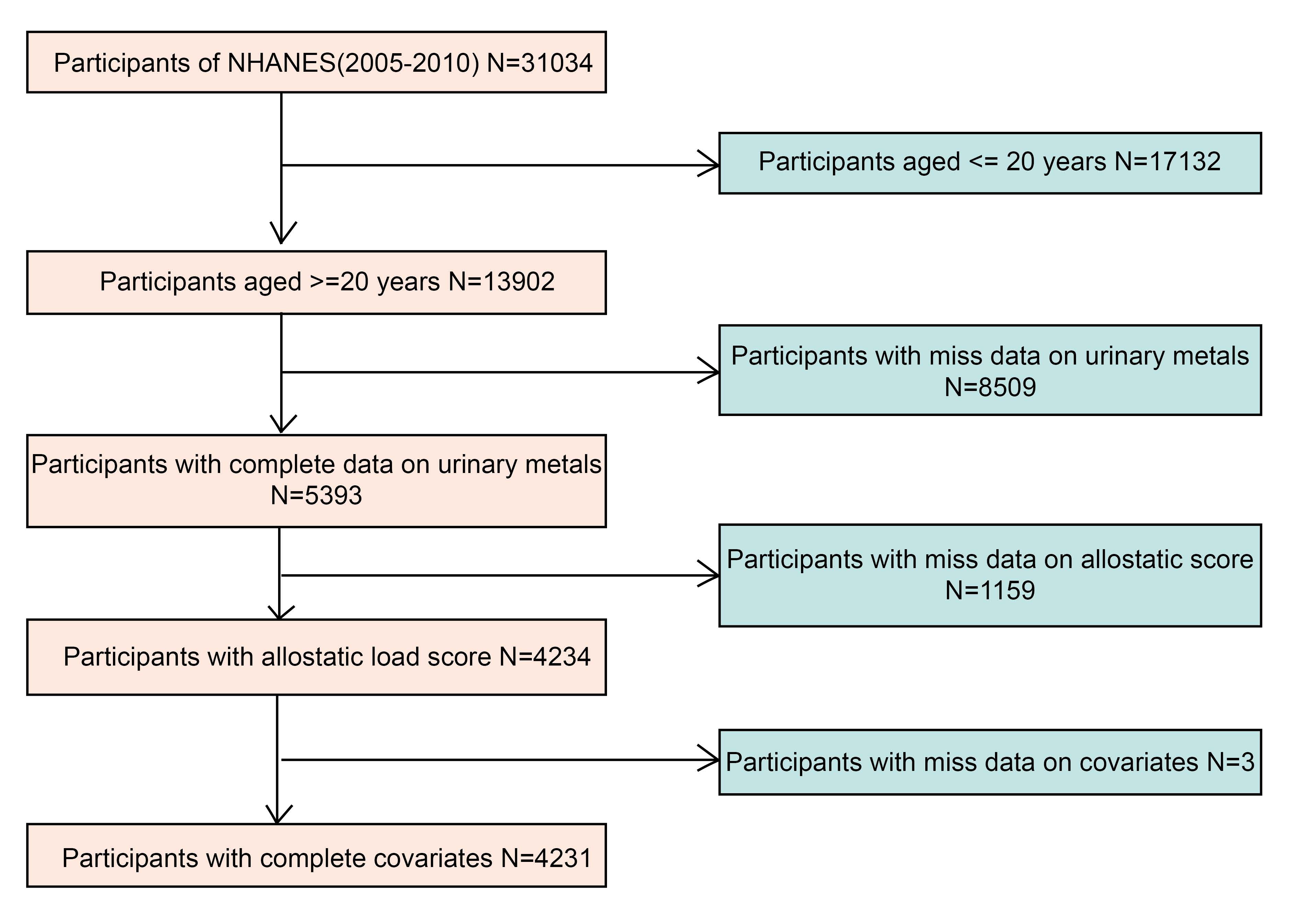
This cross-sectional study used data from 3 cycles in the NHANES website (https://www.cdc.gov/nchs/nhanes/index.htm), which was is a nationally representative study conducted by the National Center of Health Statistics comprising interviews as well as physical and medical examinations. Participants of the NHANES during the 2005 to 2010 cycles were included. Within these cycles, Measurement of urinary metals levels and all serum measurements included within our ALS calculations were completed. Measurements of C-reactive protein levels were not available in NHANES cycles after 2010. After excluding participants under 20 years old, with missing measurements included within our ALS calculations, those with missing urinary heavy metals level variables and those with missing other covariates data, 4231 participants were incorporated into the study, as illustrated in Figure 1.
Figure 1. Flow chart of the study population.
Metal measurements
The NHANES cycles between 2005 and 2010 measured the concentrations of 12 metals in urine, including Ba, Be, Cd, Co, Cs, Pt, Mo, Pb, Sb, Tl, W, and U. Methods for determining these metal concentrations are documented on the NHANES laboratory methods webpage. Natural logarithm (In) transformations were performed for 12 metal variables to maintain a normal distribution for subsequent analyses. Values below the limit of detection (LOD) are not discarded in order to maintain data integrity.Meanwhile, to account for urine dilution, all metal concentrations were adjusted for creatinine concentration, with the corrected unit measured in μg/g creatinine.
Allostatic Load Score
The biomarkers were the most commonly used in prior studies evaluating ALS and represent certain functional organ systems [7] . For the cardiovascular system, systolic and diastolic blood pressure and total serum cholesterol and high-density lipoprotein (HDL) cholesterol levels were included. For the metabolic system, levels of glycohemoglobin (hemoglobin A1c) and albumin and body mass index (calculated as weight in kilograms divided by height in meters squared) were included. Lastly, for the immune system, levels of C-reactive protein were included. As a primary analysis, based on guidance from Duong [7] , ALS was calculated by turning each biomarker into a dichotomous variable based on the statistical distribution of the sample (quartiles). One point was given if the biomarker was in the high-risk range (highest quartile) and if not (lowest 3 quartiles) with the exception of albumin and HDL cholesterol levels. For these 2 variables, a lower score indicated higher risk; thus, 1 point was given for being in the lowest quartile. In the sensitivity analysis, we also categorized each biomarker based on clinical cut points, with 1 point given if the biomarker was in the high-risk range. [15] [16] [6] Individual biomarker thresholds for clinical cut point ALS determination are listed in Table 1. Overall, possible ALS ranged between 0 and 8, and the higher the ALS, the greater the association of stress with physiologic dysregulation.
Covariates
From within the NHANES interview assessments, we included several covariates, including age (continuous in years), sex (male and female), race and ethnicity (non-Hispanic Black, non-Hispanic White, other Hispanic, and other race [includingmultiracial] ), education (less than high school, high school graduate or equivalent, some college education, or college graduate and greater), marital status (married or living with a partner or other, including widowed, divorced, separated, or never married). Smoking status was defined based on 2 self-reported questions: (1) “smoked at least 100 cigarettes in life” and (2) “Do you now smoke cigarettes?” Participants were categorized as non-smoker (answer of “no” to question 1), former smoker (answer of “yes” to question 1 but “not at all” to question 2), or current smoker (answer of “yes” to question 1 and “every day” or “some days” question 2).
Statistical analyses
The statistical software R (version 4.3.3) was utilized for the aforementioned analysis, with all significance levels set at P < 0.05 (two-tailed). Continuous or categorical variables were presented as medians and standard deviation (SD), or numerical and frequency distribution. Prior to any analysis, a logarithmic transformation of metals content in urine was performed.
We conducted weighted linear regression model to evaluate the relationship between urinary metals and allostatic load score. In this model, age, gender, education level, race, marital status, and smoking was adjusted. The results of p values were expressed.
Weighted quantile sum (WQS) and Quantile g-computation (qgcomp)
To examine the combined impacts using parametric inference, the qgcomp and WQS approach can be employed. WQS is a statistical technique used for analyzing high-dimensional data sets through multiple regression. [17] we conducted WQS analysis to assess the combined and individual impacts of heavy metals mixtures on allostatic load score by calculating a weighted linear index and assigning corresponding weights. In this study, we used bootstrapping with 1,000 iterations to construct WQS indexes in both positive and negative directions. When the WQS index was significant, corresponding weights were examined to identify the relative contribution of each heavy metal within the index to the prevalence of sarcopenia. The dataset was randomly divided, with 40% of the data allocated to the training set and the remaining 60% served as the validation set.
Qgcomp integrates the inferential framework of WQS regression with the flexibility of g-computation, addressing issues related to directional homogeneity and allowing for nonlinearity and no additivity in BKMR, thereby yielding more robust results [18] . In this study, we utilized the qgcomp model to evaluate the joint effect of exposure to a mixture of urinary metals on ALS and present both positive and negative weights for each metal in the urinary metals mixture.
Bayesian kernel machine regression (BKMR)
BKMR possesses the capacity to assess the impact of a combination of pollutants on health, as well as to estimate total exposure, individual exposure effects, and chemical interactions [19] [20] . In this study, we conducted a comparison of metals levels in urine samples collected at various percentiles and at the median in order to evaluate their overall influence on Allostatic Load Score. Additionally, we examined the specific effect of individual metals content in urine when other metals content is held constant at different percentiles. Furthermore, we explored the relationship between metals exposure and Allostatic Load Score, including any nonlinear associations. Lastly, Spearman correlation coefficients were computed to assess correlations between metals.
Machine learning component and performance evaluation
we compared the eight different machine learning algorithms including Extreme Gradient Boosting (XGBoost), Random Forest (RF), and K-Nearest Neighbors (KNN). In the comparison of the three algorithms, RF was the best choice.
RF which Breiman proposed [21] is one of the most widely used machine learning techniques. The essence of the RF algorithm is an improvement of the decision tree algorithm, and it can handle a large number of input variables. It has relatively high accuracy, robustness, and user-friendly nature. Two simple approaches for selecting features include mean decrease impurity and mean decrease accuracy [22] [23] . In addition, RF can be used to predict continuous variables and obtain predictions without obvious deviations. [24] [25]
With the test dataset, model performance was evaluated by the root-mean-square error (RMSE) expressed as
RMSE is the variance of the difference data to measure the “average error.”
Results
Participant characteristics
A total of 4231 participants from the NHANES study conducted between 2005 and 2010 were included. Medians and interquartile ranges (IQR) were calculated for the level of allostatic load score. Table 1 presents their baseline characteristics. Significant differences(P<0.05) were observed between the groups with different allostatic load score in terms of age, gender, race/ethnicity, education level, marital status, and smoking status. Furthermore, substantial differences were found in the urinary concentrations (μg/g creatinine) of heavy metals such as Be, Cd, Co, Cs, Mo, Pt, and Tl.
Table1. Baseline characteristics of participants
|
**ALS score quartiles** |
|
||||||
|
Characteristic |
Overall, N = 4231(100%)1 |
Q1, N = 1429(39%)1 |
Q2, N = 900(21%)1 |
Q3, N = 1404(30%)1 |
Q4, N = 498(9.5%)1 |
p-value2 |
|
|
Age |
46.00±16.37 |
39.00±15.55 |
46.00±16.03 |
51.00±16.08 |
53.00±14.09 |
<0.001 |
|
|
Gender |
|
|
|
|
|
0.7 |
|
|
1 |
2,122(49%) |
707(48%) |
454(50%) |
713(51%) |
248(49%) |
|
|
|
2 |
2,109(51%) |
722(52%) |
446(50%) |
691(49%) |
250(51%) |
|
|
|
Race |
|
|
|
|
|
<0.001 |
|
|
1 |
794(8.6%) |
262(8.2%) |
177(9.1%) |
260(8.6%) |
95(9.3%) |
|
|
|
2 |
381(4.5%) |
124(4.1%) |
85(5.4%) |
118(3.9%) |
54(6.1%) |
|
|
|
3 |
2,113(72%) |
787(75%) |
434(70%) |
690(72%) |
202(64%) |
|
|
|
4 |
774(10%) |
184(6.9%) |
162(9.9%) |
292(12%) |
136(18%) |
|
|
|
5 |
169(5.0%) |
72(6.2%) |
42(5.5%) |
44(3.8%) |
11(3.3%) |
|
|
|
Education level |
|
|
|
|
|
<0.001 |
|
|
1 |
542(6.8%) |
127(4.6%) |
125(7.5%) |
203(8.0%) |
87(11%) |
|
|
|
2 |
709(13%) |
209(11%) |
144(13%) |
244(13%) |
112(19%) |
|
|
|
3 |
979(24%) |
320(22%) |
210(24%) |
342(27%) |
107(23%) |
|
|
|
4 |
1,175(30%) |
392(29%) |
245(29%) |
398(32%) |
140(33%) |
|
|
|
5 |
826(26%) |
381(34%) |
176(27%) |
217(20%) |
52(14%) |
|
|
|
DMDMARTL |
|
|
|
|
|
<0.001 |
|
|
1 |
2,302(58%) |
753(54%) |
498(60%) |
799(62%) |
252(56%) |
|
|
|
2 |
345(5.5%) |
54(2.8%) |
81(5.7%) |
148(7.9%) |
62(8.7%) |
|
|
|
3 |
425(10%) |
132(9.6%) |
71(8.7%) |
153(11%) |
69(15%) |
|
|
|
4 |
147(2.5%) |
47(2.7%) |
35(2.9%) |
47(2.1%) |
18(1.8%) |
|
|
|
5 |
656(16%) |
305(21%) |
125(13%) |
167(11%) |
59(13%) |
|
|
|
6 |
356(8.7%) |
138(10%) |
90(10%) |
90(6.6%) |
38(6.0%) |
|
|
|
Smoking status |
|
|
|
|
|
0.014 |
|
|
1 |
922(23%) |
348(25%) |
186(23%) |
257(18%) |
131(27%) |
|
|
|
2 |
1,102(26%) |
322(23%) |
229(26%) |
417(30%) |
134(28%) |
|
|
|
3 |
2,207(51%) |
759(52%) |
485(52%) |
730(52%) |
233(45%) |
|
|
|
Ba |
-1.83±0.39 |
-1.82±0.38 |
-1.83±0.37 |
-1.86±0.40 |
-1.84±0.42 |
0.3 |
|
|
Be |
-3.32±0.33 |
-3.30±0.34 |
-3.31±0.34 |
-3.35±0.31 |
-3.37±0.27 |
<0.001 |
|
|
Cd |
-2.63±0.37 |
-2.69±0.37 |
-2.60±0.37 |
-2.60±0.36 |
-2.56±0.36 |
<0.001 |
|
|
Co |
-2.47±0.29 |
-2.47±0.28 |
-2.45±0.29 |
-2.49±0.30 |
-2.50±0.27 |
0.034 |
|
|
Cs |
-1.35±0.21 |
-1.35±0.21 |
-1.34±0.22 |
-1.36±0.21 |
-1.38±0.19 |
0.006 |
|
|
Mo |
-0.38±0.28 |
-0.36±0.26 |
-0.38±0.29 |
-0.41±0.29 |
-0.38±0.27 |
<0.001 |
|
|
Pb |
-2.28±0.29 |
-2.31±0.28 |
-2.26±0.31 |
-2.27±0.30 |
-2.27±0.28 |
0.10 |
|
|
Pt |
-4.22±0.39 |
-4.19±0.39 |
-4.19±0.38 |
-4.25±0.40 |
-4.27±0.43 |
<0.001 |
|
|
Sb |
-3.24±0.29 |
-3.23±0.30 |
-3.23±0.30 |
-3.24±0.28 |
-3.24±0.29 |
0.4 |
|
|
Tl |
-2.83±0.22 |
-2.81±0.22 |
-2.82±0.23 |
-2.85±0.22 |
-2.88±0.19 |
<0.001 |
|
|
W |
-3.12±0.36 |
-3.11±0.36 |
-3.09±0.38 |
-3.13±0.35 |
-3.12±0.36 |
0.4 |
|
|
U |
-4.22±0.38 |
-4.23±0.38 |
-4.22±0.39 |
-4.23±0.39 |
-4.18±0.38 |
0.13 |
|
|
1median (SD) for continuous; n(%) for categorical |
|||||||
|
2Wilcoxon rank-sum test for complex survey samples; chi-squared test with Rao & Scott's second-order correction |
|||||||
Heavy metals exposure and allostatic load score in the multivariate linear regression
To assess the potential link between log10-transformed heavy metals concentrations and the allostatic load score, we employed multivariate linear regression model which was showed in Table 2. It is worth noting that exp(Beta) means when X goes up by 1, the expected value of Y changes by about e exp(Beta). From the positive and negative values of exp(Beta) we can see the relationship between X and Y very well. Comparing with model l, there was a higher correlation between metals and allostatic load score after adjusting other heavy metals. It indicates that there may be interaction or a possible co-exposure pattern between mixed heavy metals. Meanwhile, After controlling for all confounders, the association between Be, Cd, Co, Cs, Mo, Pb, Pt, Sb and Tl and allostatic load score showed significance in multivariate linear regression(P<0.05), and were positively correlated with ALS. In the adjusted model, the risk of high allostatic load score decreased by 33.28% (exp (Beta): -1.1; 95% CI: -1.4, -0.77) for one-unit decrease in Cs concentration.
Table 2. Multivariate linear regression analysis of Log10-transformed heavy metals for allostatic load score. The crude model did not adjust for any covariates. Adjusted model I was adjusted for all covariates. Adjusted model II was adjusted for all covariates and other heavy metals.
|
|
Crude model |
Adjusted model I |
Adjusted model II |
||||||
|
|
exp(Beta) |
95%CI |
p-value |
exp(Beta) |
95%CI |
p-value |
exp(Beta) |
95%CI |
p-value |
|
Ba |
1.07 |
0.88,1.29 |
0.478 |
1.22 |
1.02,1.46 |
0.026 |
-0.11 |
-0.27, 0.04 |
0.148 |
|
Be |
0.76 |
0.58,0.99 |
0.038 |
0.77 |
0.59,1.02 |
0.058 |
-0.66 |
-0.83,-0.49 |
<0.001 |
|
Cd |
1.92 |
1.50,2.46 |
<0.001 |
0.92 |
0.72,1.18 |
0.498 |
-0.31 |
-0.57, -0.06 |
0.013 |
|
Co |
0.84 |
0.66,1.06 |
0.127 |
0.8 |
0.62,1.04 |
0.082 |
-0.51 |
-0.71, -0.31 |
<0.001 |
|
Cs |
0.8 |
0.53,1.22 |
0.292 |
0.58 |
0.39,0.86 |
0.005 |
-1.1 |
-1.4, -0.77 |
<0.001 |
|
Mo |
0.78 |
0.62,1.00 |
0.041 |
0.69 |
0.55,0.88 |
0.002 |
-0.56 |
-0.76, -0.35 |
<0.001 |
|
Pb |
1.23 |
0.98,1.53 |
0.059 |
0.71 |
0.57,0.88 |
0.001 |
-0.63 |
-0.85, -0.42 |
<0.001 |
|
Pt |
0.93 |
0.70,1.24 |
0.607 |
0.85 |
0.64,1.14 |
0.264 |
-0.51 |
-0.71, -0.31 |
<0.001 |
|
Sb |
0.89 |
0.71,1.13 |
0.326 |
1 |
0.78,1.27 |
0.964 |
-0.31 |
-0.53, -0.09 |
0.005 |
|
Tl |
0.54 |
0.37,0.79 |
<0.001 |
0.87 |
0.61,1.23 |
0.408 |
-0.84 |
-1.1, -0.56 |
<0.001 |
|
W |
0.97 |
0.77,1.21 |
0.761 |
1.04 |
0.86,1.26 |
0.678 |
-0.16 |
-0.33, 0.02 |
0.065 |
|
U |
1.02 |
0.85,1.22 |
0.833 |
1.01 |
0.86,1.18 |
0.886 |
-0.12 |
-0.28, 0.03 |
0.11 |
Heavy metals exposure and allostatic load score in WQS and qgcomp model
Both the WQS and qgcomp models were employed to estimate the weights of each metal in the mixture's overall effect. The interpretation of the results of the WQS model is based on the weighted quantile and (WQS) regression coefficients, reflecting the overall effect of the mixed exposure. The weights represent the relative contributions of each component in the mixed exposure and are used to identify the most important component in the mixed exposure (through the weight magnitude).We applied the WQS model to examine the association between the combined effects of the twelve heavy metals and the allostatic load score. The WQS index of the urinary metals was negatively associated with ALS in total.(Estimate: -0.386; P< 0.001) Figure 2A and Table 3 presented that Pb received the highest weight 0.181 for allostatic load score, followed by weight 0.177 for Cs, weight 0.145 for Mo, weight 0.125 for Pt, weight 0.7180 for Co, and in the negative direction after adjusting for all covariates. The WQS regression in the positive direction did not show any significant association of the heavy metals mixtures with allostatic load score. It is important to note that the WQS model cannot account for the effect of the direction of action of each component in the mixed exposure on the population. So we then use the qgomp model, whose results are interpreted based on the overall effect of the mixed exposure, allowing different components to have different effects in different directions, and can be used to assess the net effect of the mixed exposure (taking into account both positive and negative effects). The qgcomp model results further substantiated this finding, determining that the influence of these four heavy metals on the overall effect was negative. ( Figure 2B)
Figure 2. WQS and qgcomp models. (A)WQS weights in the WQS regression model between ALS and WQS index of heavy metal mixtures. (B) Qgcomp model regression index weights for urinary heavy metals and ALS. The model adjusted for all covariates. Ba, Barium; Be, Beryllium; Cd, Cadmium; Co, Cobalt; Cs, Cesium; Mo, Molybdenum; Pb, lead; Pt, Platinum; Sb, Antimony; Tl, Thallium; W, Tungsten; U, Uranium.
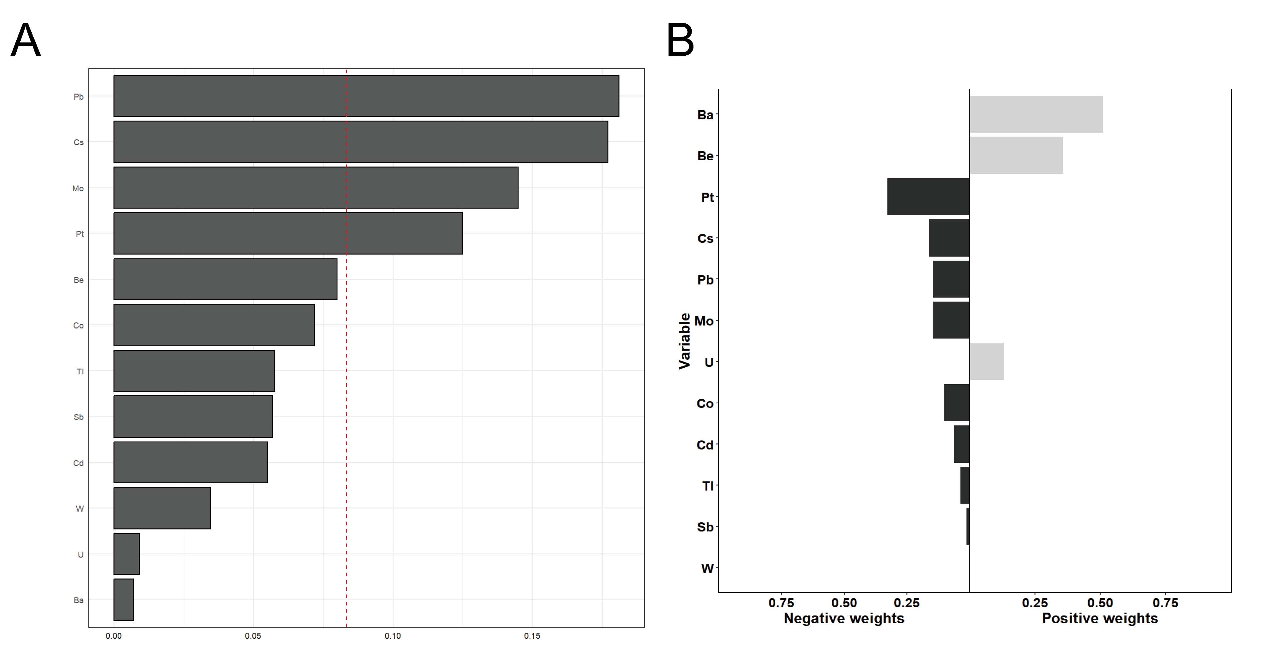
Table 3. WQS weights in the WQS regression model between ALS and WQS index of heavy metal mixtures. The model adjusted for all covariates. Ba, Barium; Be, Beryllium; Cd, Cadmium; Co, Cobalt; Cs, Cesium; Mo, Molybdenum; Pb, lead; Pt, Platinum; Sb, Antimony; Tl, Thallium; Tu, Tungsten; Ur, Uranium.
|
Mix name |
mean weight |
|
Pb |
0.18100 |
|
Cs |
0.17700 |
|
Mo |
0.14500 |
|
Pt |
0.12500 |
|
Be |
0.07990 |
|
Co |
0.07180 |
|
Tl |
0.05760 |
|
Sb |
0.05690 |
|
Cd |
0.05520 |
|
W |
0.03460 |
|
U |
0.00922 |
|
Ba |
0.00703 |
Heavy Metal Correlations in the Spearman correlation matrix
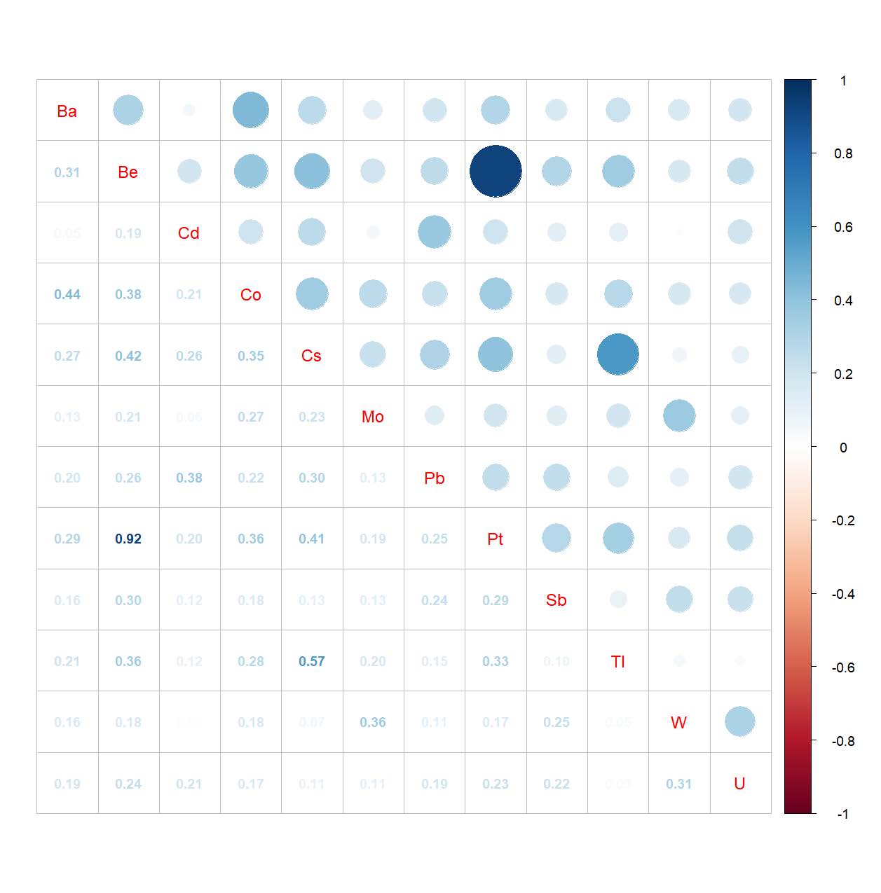
Figure 3 is a heatmap showing the correlations among the 12 heavy metals using a Spearman correlation matrix. A complex exposure profile was observed among metal concentrations, with pairwise Spearman correlations ranging from slightly positive (P= 0.02) to strong positive correlations (P = 0.92). Of the all unique pairwise correlations, the strongest correlation is between urinary platinum and beryllium (P = 0.92), which presents high relation. Besides, urinary cesium and thallium present significantly (P = 0.57).
Figure 3. Spearman correlations among the mixed exposure of twelve metals in the participants.
Heavy metals exposure and allostatic load score in BKMR model
In the BKMR model, allostatic load score was decreased for co-exposure to heavy metals mixtures above the 50th percentile compared to the medians. Figure 4A shows the overall exposure-response function trend of 12 heavy metals. When the other 11 metals were fixed at the median level, the univariate exposure-response relationship showed Cs, Pt, Pb, Co and Mo have a downward trend with ALS, with non-linear relationship. Notably, the univariate exposure–response curve for Cs and Pt is steeper than that for other three metals. The other seven metals do not show obvious ALS relationship. (Figure 4B).
Figure 4. BKMR model. (A) Overall effect of metals in urine and ALS based on BKMR. (B)Univariate exposure–response function between each heavy metals and ALS when the other heavy metals were fixed at 50th percentiles. (C) Bivariate exposure-response relationship between twelve urinary heavy metals and ALS (a visualization for evaluating interactions).The model adjusted for all covariates. Ba, Barium; Be, Beryllium; Cd, Cadmium; Co, Cobalt; Cs, Cesium; Mo, Molybdenum; Pb, lead; Pt, Platinum; Sb, Antimony; Tl, Thallium; W, Tungsten; U, Uranium.
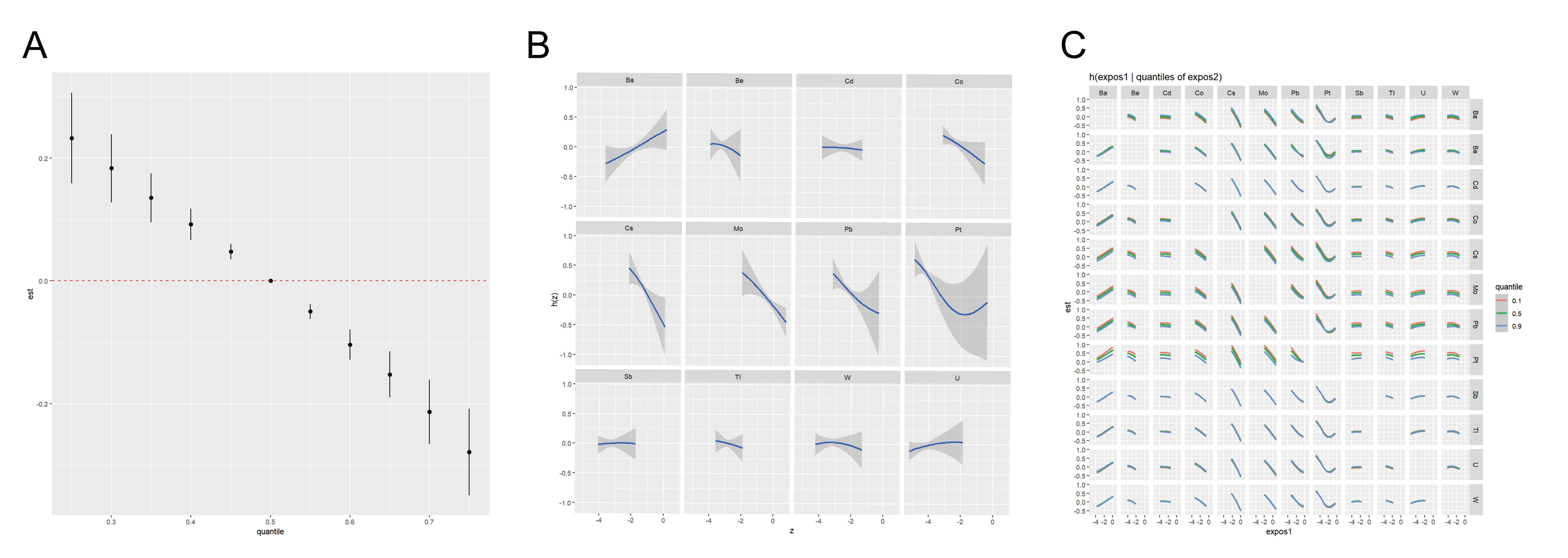
Table 4 shows higher estimated PIPs for Cs (PIP = 1.0000), Pt (PIP = 1.0000), Mo (PIP = 0.9384), Co (PIP = 0.9272) Pb (PIP=0.9088), consistent with the previous two models. We further explored heavy metal interactions (Figure 4C). We fixed the other heavy metals at the median level and determined the exposure-response function of one heavy metal to a second heavy metal at its 10th, 50th, and 90th percentiles, respectively. No evidence of chemical interaction was found among each two of these heavy metals.
Table 4. The posteriori inclusion probability of single urinary metals
Evaluation and comparison of the ML model
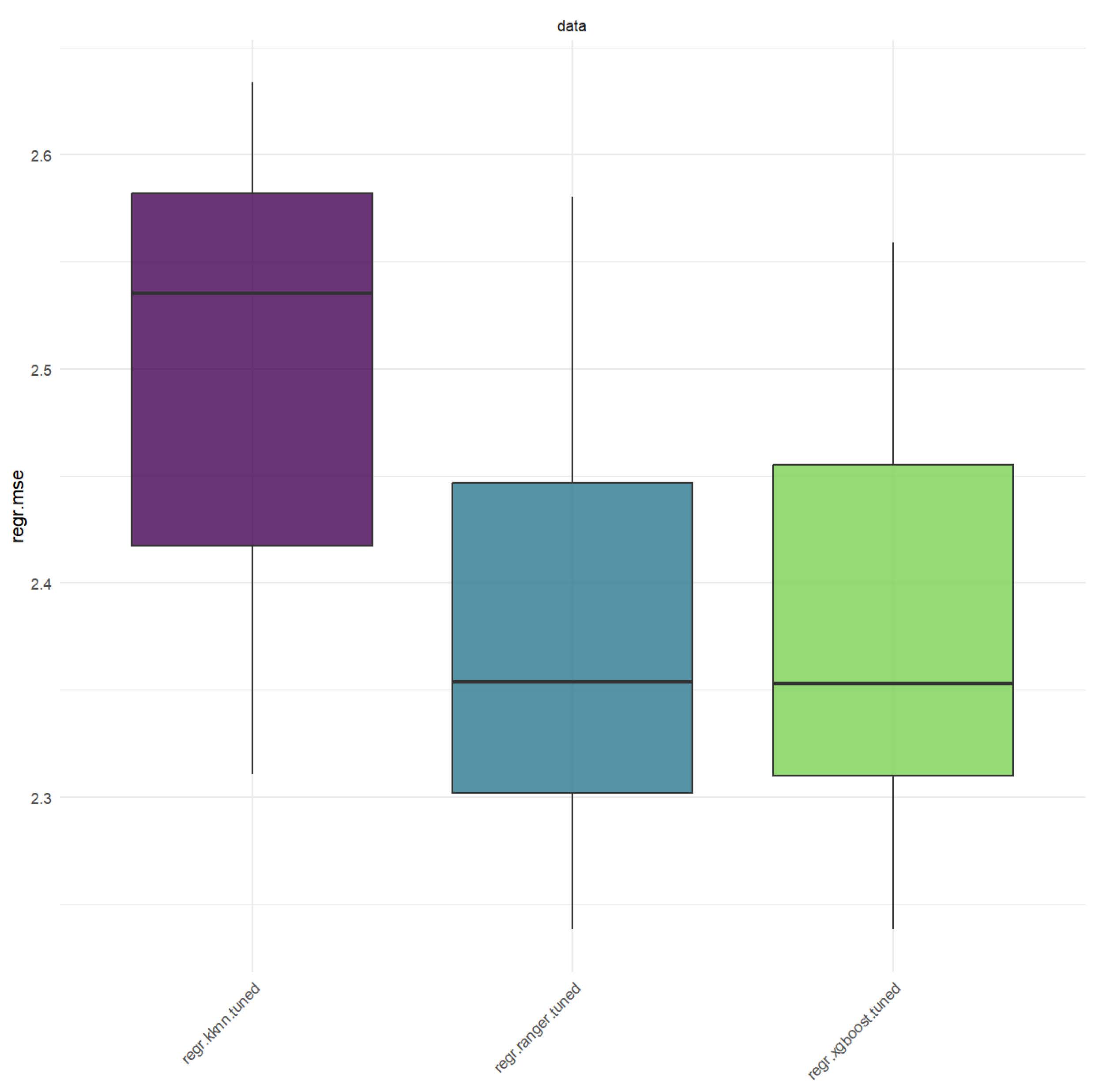
Figure. 5 depicts three ML models. The study used 10-fold cross-validation to divide the entire sample into 10 equally sized subsamples. Among the 10 subsamples, one was retained as the verification data set of the test model, and the remaining nine were used as the training data set. After the cross-validation process was repeated 10 times, 10 results were generated, and the average value was taken as the performance metric. In this paper, the Root Mean Absolute Error (RMAE) was selected as the evaluation index.
Comparing the prediction performance of the RF, KNN and XGBoost prediction model, in terms of the Root Mean Absolute Error (RMAE), the RMAE of the RF prediction model was 2.377428, the RMAE of the KNN model was 2.501523 and the RMAE of the XGBoost model was 2.377733. Respectively. The prediction accuracy of the RF prediction model was best in three model (Table 1). The results were also shown in Figure 5.
Figure 5. Three ML model benchmark test results.
Discussion
Allostatic load which indicates the cumulative strain associated with the chronic stress response due to repeated environmental challenges is quantified by the allostatic load score, an established measure of the cardiovascular, metabolic, and immune ramifications of stress. [7] [8] Some studies was observed that heavy metals had significant and positively associations with CVD. [2627] [28] And long-term exposure to heavy metals (either low-dose or high-dose) uniformly causes immunosuppression and directly interferes with the sensitization of the immune system to antigens [29] . However, A study based on the data of NHANES from 2005 to 2018, through WQS and BKMR models, found that the mixed metals content in urine was negatively correlated with Mets. And in the study of single metal, the contents of Cs and Pb in urine are verified to be negatively correlated with Mets through logistic regression and the BKMR model [20] .
Based on the data of NHANES from 2005 to 2010, this study analyzed twelve kinds of metals in urine and found that the mixed metals content in urine was negatively correlated with ALS through WQS and BKMR models. In the study of single metal, linear regression and the BKMR model verify that the contents of Cs, Pb, Mo and Pt in urine are negatively correlated with ALS. With the increase in metals content, allostatic load is monotonically decreasing. The result is contrary to our previous speculation. We surmise that there may be one reasons that the effect on metabolism may be the main factor between twelve urinary heavy metals and allostatic load.
According to previous research, Cs is closely related to the diagnostic factors of ALS. A study suggests that Cs are significantly related to HDL by studying chronic exposure of adult, postnatal and in utero rat models to low-dose 137 Cesium [30] . A repeated-measures study of older adults in Beijing showed that Cs were positively correlated with HDL [31] , consistent with previous research results [32] . In addition, it is found that Cs have no significant relationship with SBP but have a negative correlation with DBP [31] . A study has found a significant negative correlation between Cs and BMI by utilizing the NHANES 99-02 data [33] .
As for the mechanism behind the conclusion that the combined effect of 12 urinary metals is negatively correlated with allostatic load, we speculated that it may be related to the disruption of cell homeostasis by heavy metals such as lead, which can replace bivalent cations such as calcium and zinc, but also activate the Keap1-Nrf2 pathway. After Nrf2 enters the nucleus, it initiates the expression of genes regulated by antioxidant reaction elements (ARE), promotes the production of antioxidant enzymes such as glutathione synthetase and superoxide dismutase (SOD), and enhances the resistance of cells to oxidative stress, thus reducing the contribution of oxidative damage to adaptive load. At the same time, lead exposure induces the upregulation of endoplasmic reticulum (ER) stress proteins, such as glucose-regulating protein GRP78, and activates the unfolded protein response (UPR). Moderate UPR can repair cell function by enhancing protein folding capacity and clearing misfolded proteins, which may relieve stress load in the short term [34] .
Regarding the correlation between beryllium and platinum, it has been shown that beryllium (BeSO₄) and the platinum compound (PT-5-sulfomercaptoquinoline salt) both inhibit CA-ATPase activity in the sarcoplasmic reticulum (SR), but their inhibition is weaker than that of other compounds such as aminophenthiazine. This suggests that the two may indirectly affect each other's metabolic or excretory pathways by interfering with the activity of membrane-binding enzymes, such as those associated with calcium ion transport, which may be the reason for the correlation of composition in the urine of the two [35] .
Since machine learning algorithms were widely used in diagnosing and prediction, we tried to make a prediction of ALS. We used a machine learning algorithm suitable for large-scale data, including 4231 samples. The RF model with RMSE was 2.377428. The model could be used to predict ALS for individuals, and provided a theoretical basis for further allostatic load targeted interventions.
This study still has some limitations. First, NHANES adopts a cross-sectional design, so it cannot further judge the causal relationship between metals content in urine and ALS. Second, the participants in this study are all Americans, and the results obtained may not apply to other people. Third, NHANES uses random urine samples to detect the metal concentrations in urine, and there may be some deviations in the metals content in urine. Because ALS is a continuous variable, we just use three ML models to predict ALS and the evaluation index of the ML model is single, lacking credibility.
5. Conclusion
The analysis of NHANES data showed that the mixed effect of twelve metals in urine is negatively correlated with ALS among American adults. The contents of cesium (Cs), Molybdenum (Mo), lead (Pb), Platinum (Pt) in urine were most negatively correlated with ALS. It is hoped that there will be a cohort study in the future to expose the influence of metals on ALS, which can provide higher-level evidence. In addition, it is hoped that relevant basic research can reveal the mechanism of the occurrence and development of metals and allostatic load. Finally, we employed three ML models to establish a predictive model for ALS utilizing heavy metals exposure data from the NHANES. Among these models, the RF approach exhibited superior performance.
Acknowledgements
The data was derived from published National Health and Nutrition Examination Survey (NHANES). The authors thank all investigators for sharing these data.
Author contributions
Yiyin Rong: Conceptualization, Writing- Original draft preparation. Shenglin Luo: Data curation, Writing- Original draft preparation. Cong Wu: Methodology, Visualization. Haozhe Huang: Visualization. Validation. Ming Chen: Visualization. Xingyu Liu: Investigation. Shaobo Wu: Writing- Reviewing and Editing, Supervision.
Ethics approval and consent to participate
The studies involving human participants were reviewed and approved by the National Center for Health Statistics Research Ethics Review Board. The patients/participants provided their written informed consent to participate in this study. Written informed consent was obtained from the individual(s)for the publication of any potentially identifiable images or data included in this article.
Funding information
Not applicable.
Competing Interests
The authors declare that they have no existing or potential commercial or financial relationships that could create a conflict of interest at the time of conducting this study.
Data Availability
All data needed to evaluate the conclusions in the paper are present in the paper or the Supplementary Materials. Additional data related to this paper may be requested from the authors.
References
[1] Muhibbullah M, Haleem AMA, Ikuma Y. (2017). Frequency dependent power and energy flux density equations of the electromagnetic wave. Results in Physics.7,435-9.http://https://doi.org/10.1016/j.rinp.2017.01.006
[2] Gautam R, Singh KV, Nirala J, Murmu NN, Meena R, Rajamani P. (2019). Oxidative stress-mediated alterations on sperm parameters in male Wistar rats exposed to 3G mobile phone radiation. Andrologia.51(3),e13201.http://https://doi.org/10.1111/and.13201
[3] Verbeek J, Oftedal G, Feychting M, van Rongen E, Rosaria Scarfì M, Mann S, et al. (2021). Prioritizing health outcomes when assessing the effects of exposure to radiofrequency electromagnetic fields: A survey among experts. Environment International.146,106300.http://https://doi.org/10.1016/j.envint.2020.106300
[4] Mahaldashtian M, Khalili MA, Anbari F, Seify M, Belli M. (2022). Challenges on the effect of cell phone radiation on mammalian embryos and fetuses: a review of the literature. Zygote.30(2),176-82.http://10.1017/S0967199421000691
[5] Lagorio S, Blettner M, Baaken D, Feychting M, Karipidis K, Loney T, et al. (2021). The effect of exposure to radiofrequency fields on cancer risk in the general and working population: A protocol for a systematic review of human observational studies. Environment International.157,106828.http://https://doi.org/10.1016/j.envint.2021.106828
[6] Keleş Aİ. (2020). Morphological changes in the vertebrae and central canal of rat pups born after exposure to the electromagnetic field of pregnant rats. Acta Histochemica.122(8),151652.http://https://doi.org/10.1016/j.acthis.2020.151652
[7] Keleş Aİ, Süt BB. (2021). Histopathological and epigenetic alterations in the spinal cord due to prenatal electromagnetic field exposure: An H3K27me3-related mechanism. Toxicology and Industrial Health.37(4),189-97.http://10.1177/0748233721996947
[8] Odaci E, Bas O, Kaplan S. (2008). Effects of prenatal exposure to a 900 MHz electromagnetic field on the dentate gyrus of rats: a stereological and histopathological study. Brain Research.1238,224-9.http://https://doi.org/10.1016/j.brainres.2008.08.013
[9] Kilic A, Ustunova S, Bulut H, Meral I. (2023). Pre and postnatal exposure to 900 MHz electromagnetic fields induce inflammation and oxidative stress, and alter renin-angiotensin system components differently in male and female offsprings. Life Sciences.321,121627.http://https://doi.org/10.1016/j.lfs.2023.121627
[10] Haghani M, Shabani M, Moazzami K. (2013). Maternal mobile phone exposure adversely affects the electrophysiological properties of Purkinje neurons in rat offspring. Neuroscience.250,588-98.http://https://doi.org/10.1016/j.neuroscience.2013.07.049
[11] Feychting M, Ahlbom A, Kheifets L. (2005). EMF and health. Annu Rev Public Health.26,165-89.http://10.1146/annurev.publhealth.26.021304.144445
[12] Blaasaas KG, Tynes T, Irgens A, Lie RT. (2002). Risk of birth defects by parental occupational exposure to 50 Hz electromagnetic fields: a population based study. Occup Environ Med.59(2),92-7.http://10.1136/oem.59.2.92
[13] Baldi I, Coureau G, Jaffré A, Gruber A, Ducamp S, Provost D, et al. (2011). Occupational and residential exposure to electromagnetic fields and risk of brain tumors in adults: a case-control study in Gironde, France. Int J Cancer.129(6),1477-84.http://10.1002/ijc.25765
[14] De Roos AJ, Teschke K, Savitz DA, Poole C, Grufferman S, Pollock BH, Olshan AF. (2001). Parental occupational exposures to electromagnetic fields and radiation and the incidence of neuroblastoma in offspring. Epidemiology.12(5),508-17.http://10.1097/00001648-200109000-00008
[15] Razavinasab M, Moazzami K, Shabani M. (2016). Maternal mobile phone exposure alters intrinsic electrophysiological properties of CA1 pyramidal neurons in rat offspring. Toxicol Ind Health.32(6),968-79.http://10.1177/0748233714525497
[16] Zhang Y, Li Z, Gao Y, Zhang C. (2015). Effects of fetal microwave radiation exposure on offspring behavior in mice. J Radiat Res.56(2),261-8.http://10.1093/jrr/rru097
[17] Birks L, Guxens M, Papadopoulou E, Alexander J, Ballester F, Estarlich M, et al. (2017). Maternal cell phone use during pregnancy and child behavioral problems in five birth cohorts. Environ Int.104,122-31.http://10.1016/j.envint.2017.03.024
[18] Kumari K, Koivisto H, Capstick M, Naarala J, Viluksela M, Tanila H, Juutilainen J. (2018). Behavioural phenotypes in mice after prenatal and early postnatal exposure to intermediate frequency magnetic fields. Environ Res.162,27-34.http://10.1016/j.envres.2017.12.013
[19] Acikgoz B, Ersoy N, Aksu I, Kiray A, Bagriyanik HA, Kiray M. (2022). Gender differences in effects of prenatal and postnatal exposure to electromagnetic field and prenatal zinc on behaviour and synaptic proteins in rats. J Chem Neuroanat.122,102092.http://10.1016/j.jchemneu.2022.102092
[20] Agarwal A, Singh A, Hamada A, Kesari K. (2011). Cell phones and male infertility: a review of recent innovations in technology and consequences. Int Braz J Urol.37(4),432-54.http://10.1590/s1677-55382011000400002
[21] Ersoy N, Acikgoz B, Aksu I, Kiray A, Bagriyanik HA, Kiray M. (2022). The Effects of Prenatal and Postnatal Exposure to 50-Hz and 3 mT Electromagnetic Field on Rat Testicular Development. Medicina (Kaunas).59(1).http://10.3390/medicina59010071
[22] Özorak A, Nazıroğlu M, Çelik Ö, Yüksel M, Özçelik D, Özkaya MO, et al. (2013). Wi-Fi (2.45 GHz)- and mobile phone (900 and 1800 MHz)-induced risks on oxidative stress and elements in kidney and testis of rats during pregnancy and the development of offspring. Biol Trace Elem Res.156(1-3),221-9.http://10.1007/s12011-013-9836-z
[23] Yan S, Ju Y, Dong J, Lei H, Wang J, Xu Q, et al. (2022). Paternal Radiofrequency Electromagnetic Radiation Exposure Causes Sex-Specific Differences in Body Weight Trajectory and Glucose Metabolism in Offspring Mice. Front Public Health.10,872198.http://10.3389/fpubh.2022.872198
[24] Andrašková S, Holovská K, Ševčíková Z, Andrejčáková Z, Tóth Š, Martončíková M, et al. (2022). The potential adverse effect of 2.45 GHz microwave radiation on the testes of prenatally exposed peripubertal male rats. Histol Histopathol.37(3),287-99.http://10.14670/hh-18-402
[25] Ryan BM, Symanski RR, Pomeranz LE, Johnson TR, Gauger JR, McCormick DL. (1999). Multigeneration reproductive toxicity assessment of 60-Hz magnetic fields using a continuous breeding protocol in rats. Teratology.59(3),156-62.http://10.1002/(sici)1096-9926(199903)59:3<156::Aid-tera7>3.0.Co;2-b
[26] Burcu A, Nevin E, Ilkay A, Amac K, Alper BH, Muge K. (2020). The effects of prenatal and postnatal exposure to electromagnetic field on rat ovarian tissue. Toxicology and Industrial Health.36(12),1010-8.http://10.1177/0748233720973136
[27] Shirai T, Wang J, Kawabe M, Wake K, Watanabe S-i, Takahashi S, Fujiwara O. (2017). No adverse effects detected for simultaneous whole-body exposure to multiple-frequency radiofrequency electromagnetic fields for rats in the intrauterine and pre- and post-weaning periods. Journal of Radiation Research.58(1),48-58.http://10.1093/jrr/rrw085
[28] Takahashi S, Imai N, Nabae K, Wake K, Kawai H, Wang J, et al. (2009). Lack of Adverse Effects of Whole-Body Exposure to a Mobile Telecommunication Electromagnetic Field on the Rat Fetus. Radiation Research.173(3),362-72.http://10.1667/rr1615.1
[29] Baste V, Riise T, Moen BE. (2008). Radiofrequency electromagnetic fields; male infertility and sex ratio of offspring. European Journal of Epidemiology.23(5),369-77.http://10.1007/s10654-008-9236-4
[30] Mageroy N, Mollerlokken OJ, Riise T, Koefoed V, Moen BE. (2006). A higher risk of congenital anomalies in the offspring of personnel who served aboard a Norwegian missile torpedo boat. Occupational and Environmental Medicine.63(2),92.http://10.1136/oem.2005.021113
[31] Baste V, Moen BE, Oftedal G, Strand LÅ, Bjørge L, Mild KH. (2012). Pregnancy Outcomes After Paternal Radiofrequency Field Exposure Aboard Fast Patrol Boats. Journal of Occupational and Environmental Medicine.54(4),431-8.http://10.1097/JOM.0b013e3182445003
[32] Baste V, Oftedal G, Møllerløkken OJ, Hansson Mild K, Moen BE. (2015). Prospective Study of Pregnancy Outcomes After Parental Cell Phone Exposure: The Norwegian Mother and Child Cohort Study. Epidemiology.26(4),613-21.http://10.1097/ede.0000000000000293
[33] Knave B, Gamberale F, BergstrÖM S, Birke E, Iregren A, Kolmodin-Hedman B, Wennberg A. (1979). Long-term exposure to electric fields: A cross-sectional epidemiologic investigation of occupationally exposed workers in high-voltage substations. Scandinavian Journal of Work, Environment & Health.5(2),115-25
[34] Topal Z, Hanci H, Mercantepe T, Erol HS, Keleş ON, Kaya H, et al. (2015). The effects of prenatal long-duration exposure to 900-MHz electromagnetic field on the 21-day-old newborn male rat liver. Turk J Med Sci.45(2),291-7.http://10.3906/sag-1404-168
[35] Bozok S, Karaagac E, Sener D, Akakin D, Tumkaya L. (2022). The effects of long-term prenatal exposure to 900, 1800, and 2100 MHz electromagnetic field radiation on myocardial tissue of rats. Toxicology and Industrial Health.39(1),1-9.http://10.1177/07482337221139586
[36] Bahreyni Toossi MH, Reza SH, Maryam MMF, Mahmoud H, Mahdiyeh H, Razieh M, et al. (2018). Exposure to mobile phone (900–1800 MHz) during pregnancy: tissue oxidative stress after childbirth. The Journal of Maternal-Fetal & Neonatal Medicine.31(10),1298-303.http://10.1080/14767058.2017.1315657
[37] Guleken Z, Sarıbal D, Uyulan C, Keles A, Depciuch J. (2021). Investigating Bio-interface Effects of Chronic ELF-MF Exposure before and after Neonatal Life on Rat Offspring Using Spectroscopy and Biochemical Assays. Biointerface Research in Applied Chemistry.12(1),795 - 808.https://doi.org/10.33263/BRIAC121.795808
[38] Çiftçi ZZ, Kırzıoğlu Z, Nazıroğlu M, Özmen Ö. (2015). Effects of Prenatal and Postnatal Exposure of Wi-Fi on Development of Teeth and Changes in Teeth Element Concentration in Rats. Biological Trace Element Research.163(1),193-201.http://10.1007/s12011-014-0175-5
[39] Özorak A, Nazıroğlu M, Çelik Ö, Yüksel M, Özçelik D, Özkaya MO, et al. (2013). Wi-Fi (2.45 GHz)- and Mobile Phone (900 and 1800 MHz)-Induced Risks on Oxidative Stress and Elements in Kidney and Testis of Rats During Pregnancy and the Development of Offspring. Biological Trace Element Research.156(1),221-9.http://10.1007/s12011-013-9836-z
[40] Lary JM, Conover DL, Johnson PH, Burg JR. (1983). Teratogenicity of 27.12-MHz radiation in rats is related to duration of hyperthermic exposure. Bioelectromagnetics.4(3),249-55.https://doi.org/10.1002/bem.2250040305
[41] GÜLER ÖZTÜRK G, Tomruk A, Ozgur E, Seyhan N. (2010). The effect of radiofrequency radiation on DNA and lipid damage in non-pregnant and pregnant rabbits and their newborns. General physiology and biophysics.29(1).https://10.4149/gpb_2010_01_59
[42] Pearce MS, Hammal DM, Dorak MT, McNally RJQ, Parker L. (2007). Paternal occupational exposure to electro-magnetic fields as a risk factor for cancer in children and young adults: A case-control study from the North of England. Pediatric Blood & Cancer.49(3),280-6.https://doi.org/10.1002/pbc.21021
[43] Reid A, Glass DC, Bailey HD, Milne E, de Klerk NH, Downie P, et al. (2011). Risk of childhood acute lymphoblastic leukaemia following parental occupational exposure to extremely low frequency electromagnetic fields. British Journal of Cancer.105(9),1409-13.http://10.1038/bjc.2011.365
[44] Bohacek J, Mansuy IM. (2015). Molecular insights into transgenerational non-genetic inheritance of acquired behaviours. Nature Reviews Genetics.16(11),641-52.http://10.1038/nrg3964
[45] Cavalli G, Heard E. (2019). Advances in epigenetics link genetics to the environment and disease. Nature.571(7766),489-99.http://10.1038/s41586-019-1411-0
[46] Nagano T, Lubling Y, Stevens TJ, Schoenfelder S, Yaffe E, Dean W, et al. (2013). Single-cell Hi-C reveals cell-to-cell variability in chromosome structure. Nature.502(7469),59-64.http://10.1038/nature12593
 Figures
 References
 Peer
Peer Information
Figure 1. Flow chart of the study population.
Figure 2. WQS and qgcomp models. (A)WQS weights in the WQS regression model between ALS and WQS index of heavy metal mixtures. (B) Qgcomp model regression index weights for urinary heavy metals and ALS. The model adjusted for all covariates. Ba, Barium; Be, Beryllium; Cd, Cadmium; Co, Cobalt; Cs, Cesium; Mo, Molybdenum; Pb, lead; Pt, Platinum; Sb, Antimony; Tl, Thallium; W, Tungsten; U, Uranium.
Figure 3. Spearman correlations among the mixed exposure of twelve metals in the participants.
Figure 4. BKMR model. (A) Overall effect of metals in urine and ALS based on BKMR. (B)Univariate exposure–response function between each heavy metals and ALS when the other heavy metals were fixed at 50th percentiles. (C) Bivariate exposure-response relationship between twelve urinary heavy metals and ALS (a visualization for evaluating interactions).The model adjusted for all covariates. Ba, Barium; Be, Beryllium; Cd, Cadmium; Co, Cobalt; Cs, Cesium; Mo, Molybdenum; Pb, lead; Pt, Platinum; Sb, Antimony; Tl, Thallium; W, Tungsten; U, Uranium.
Figure 5. Three ML model benchmark test results.
[1] Muhibbullah M, Haleem AMA, Ikuma Y. (2017). Frequency dependent power and energy flux density equations of the electromagnetic wave. Results in Physics.7,435-9.http://https://doi.org/10.1016/j.rinp.2017.01.006
[2] Gautam R, Singh KV, Nirala J, Murmu NN, Meena R, Rajamani P. (2019). Oxidative stress-mediated alterations on sperm parameters in male Wistar rats exposed to 3G mobile phone radiation. Andrologia.51(3),e13201.http://https://doi.org/10.1111/and.13201
[3] Verbeek J, Oftedal G, Feychting M, van Rongen E, Rosaria Scarfì M, Mann S, et al. (2021). Prioritizing health outcomes when assessing the effects of exposure to radiofrequency electromagnetic fields: A survey among experts. Environment International.146,106300.http://https://doi.org/10.1016/j.envint.2020.106300
[4] Mahaldashtian M, Khalili MA, Anbari F, Seify M, Belli M. (2022). Challenges on the effect of cell phone radiation on mammalian embryos and fetuses: a review of the literature. Zygote.30(2),176-82.http://10.1017/S0967199421000691
[5] Lagorio S, Blettner M, Baaken D, Feychting M, Karipidis K, Loney T, et al. (2021). The effect of exposure to radiofrequency fields on cancer risk in the general and working population: A protocol for a systematic review of human observational studies. Environment International.157,106828.http://https://doi.org/10.1016/j.envint.2021.106828
[6] Keleş Aİ. (2020). Morphological changes in the vertebrae and central canal of rat pups born after exposure to the electromagnetic field of pregnant rats. Acta Histochemica.122(8),151652.http://https://doi.org/10.1016/j.acthis.2020.151652
[7] Keleş Aİ, Süt BB. (2021). Histopathological and epigenetic alterations in the spinal cord due to prenatal electromagnetic field exposure: An H3K27me3-related mechanism. Toxicology and Industrial Health.37(4),189-97.http://10.1177/0748233721996947
[8] Odaci E, Bas O, Kaplan S. (2008). Effects of prenatal exposure to a 900 MHz electromagnetic field on the dentate gyrus of rats: a stereological and histopathological study. Brain Research.1238,224-9.http://https://doi.org/10.1016/j.brainres.2008.08.013
[9] Kilic A, Ustunova S, Bulut H, Meral I. (2023). Pre and postnatal exposure to 900 MHz electromagnetic fields induce inflammation and oxidative stress, and alter renin-angiotensin system components differently in male and female offsprings. Life Sciences.321,121627.http://https://doi.org/10.1016/j.lfs.2023.121627
[10] Haghani M, Shabani M, Moazzami K. (2013). Maternal mobile phone exposure adversely affects the electrophysiological properties of Purkinje neurons in rat offspring. Neuroscience.250,588-98.http://https://doi.org/10.1016/j.neuroscience.2013.07.049
[11] Feychting M, Ahlbom A, Kheifets L. (2005). EMF and health. Annu Rev Public Health.26,165-89.http://10.1146/annurev.publhealth.26.021304.144445
[12] Blaasaas KG, Tynes T, Irgens A, Lie RT. (2002). Risk of birth defects by parental occupational exposure to 50 Hz electromagnetic fields: a population based study. Occup Environ Med.59(2),92-7.http://10.1136/oem.59.2.92
[13] Baldi I, Coureau G, Jaffré A, Gruber A, Ducamp S, Provost D, et al. (2011). Occupational and residential exposure to electromagnetic fields and risk of brain tumors in adults: a case-control study in Gironde, France. Int J Cancer.129(6),1477-84.http://10.1002/ijc.25765
[14] De Roos AJ, Teschke K, Savitz DA, Poole C, Grufferman S, Pollock BH, Olshan AF. (2001). Parental occupational exposures to electromagnetic fields and radiation and the incidence of neuroblastoma in offspring. Epidemiology.12(5),508-17.http://10.1097/00001648-200109000-00008
[15] Razavinasab M, Moazzami K, Shabani M. (2016). Maternal mobile phone exposure alters intrinsic electrophysiological properties of CA1 pyramidal neurons in rat offspring. Toxicol Ind Health.32(6),968-79.http://10.1177/0748233714525497
[16] Zhang Y, Li Z, Gao Y, Zhang C. (2015). Effects of fetal microwave radiation exposure on offspring behavior in mice. J Radiat Res.56(2),261-8.http://10.1093/jrr/rru097
[17] Birks L, Guxens M, Papadopoulou E, Alexander J, Ballester F, Estarlich M, et al. (2017). Maternal cell phone use during pregnancy and child behavioral problems in five birth cohorts. Environ Int.104,122-31.http://10.1016/j.envint.2017.03.024
[18] Kumari K, Koivisto H, Capstick M, Naarala J, Viluksela M, Tanila H, Juutilainen J. (2018). Behavioural phenotypes in mice after prenatal and early postnatal exposure to intermediate frequency magnetic fields. Environ Res.162,27-34.http://10.1016/j.envres.2017.12.013
[19] Acikgoz B, Ersoy N, Aksu I, Kiray A, Bagriyanik HA, Kiray M. (2022). Gender differences in effects of prenatal and postnatal exposure to electromagnetic field and prenatal zinc on behaviour and synaptic proteins in rats. J Chem Neuroanat.122,102092.http://10.1016/j.jchemneu.2022.102092
[20] Agarwal A, Singh A, Hamada A, Kesari K. (2011). Cell phones and male infertility: a review of recent innovations in technology and consequences. Int Braz J Urol.37(4),432-54.http://10.1590/s1677-55382011000400002
[21] Ersoy N, Acikgoz B, Aksu I, Kiray A, Bagriyanik HA, Kiray M. (2022). The Effects of Prenatal and Postnatal Exposure to 50-Hz and 3 mT Electromagnetic Field on Rat Testicular Development. Medicina (Kaunas).59(1).http://10.3390/medicina59010071
[22] Özorak A, Nazıroğlu M, Çelik Ö, Yüksel M, Özçelik D, Özkaya MO, et al. (2013). Wi-Fi (2.45 GHz)- and mobile phone (900 and 1800 MHz)-induced risks on oxidative stress and elements in kidney and testis of rats during pregnancy and the development of offspring. Biol Trace Elem Res.156(1-3),221-9.http://10.1007/s12011-013-9836-z
[23] Yan S, Ju Y, Dong J, Lei H, Wang J, Xu Q, et al. (2022). Paternal Radiofrequency Electromagnetic Radiation Exposure Causes Sex-Specific Differences in Body Weight Trajectory and Glucose Metabolism in Offspring Mice. Front Public Health.10,872198.http://10.3389/fpubh.2022.872198
[24] Andrašková S, Holovská K, Ševčíková Z, Andrejčáková Z, Tóth Š, Martončíková M, et al. (2022). The potential adverse effect of 2.45 GHz microwave radiation on the testes of prenatally exposed peripubertal male rats. Histol Histopathol.37(3),287-99.http://10.14670/hh-18-402
[25] Ryan BM, Symanski RR, Pomeranz LE, Johnson TR, Gauger JR, McCormick DL. (1999). Multigeneration reproductive toxicity assessment of 60-Hz magnetic fields using a continuous breeding protocol in rats. Teratology.59(3),156-62.http://10.1002/(sici)1096-9926(199903)59:3<156::Aid-tera7>3.0.Co;2-b
[26] Burcu A, Nevin E, Ilkay A, Amac K, Alper BH, Muge K. (2020). The effects of prenatal and postnatal exposure to electromagnetic field on rat ovarian tissue. Toxicology and Industrial Health.36(12),1010-8.http://10.1177/0748233720973136
[27] Shirai T, Wang J, Kawabe M, Wake K, Watanabe S-i, Takahashi S, Fujiwara O. (2017). No adverse effects detected for simultaneous whole-body exposure to multiple-frequency radiofrequency electromagnetic fields for rats in the intrauterine and pre- and post-weaning periods. Journal of Radiation Research.58(1),48-58.http://10.1093/jrr/rrw085
[28] Takahashi S, Imai N, Nabae K, Wake K, Kawai H, Wang J, et al. (2009). Lack of Adverse Effects of Whole-Body Exposure to a Mobile Telecommunication Electromagnetic Field on the Rat Fetus. Radiation Research.173(3),362-72.http://10.1667/rr1615.1
[29] Baste V, Riise T, Moen BE. (2008). Radiofrequency electromagnetic fields; male infertility and sex ratio of offspring. European Journal of Epidemiology.23(5),369-77.http://10.1007/s10654-008-9236-4
[30] Mageroy N, Mollerlokken OJ, Riise T, Koefoed V, Moen BE. (2006). A higher risk of congenital anomalies in the offspring of personnel who served aboard a Norwegian missile torpedo boat. Occupational and Environmental Medicine.63(2),92.http://10.1136/oem.2005.021113
[31] Baste V, Moen BE, Oftedal G, Strand LÅ, Bjørge L, Mild KH. (2012). Pregnancy Outcomes After Paternal Radiofrequency Field Exposure Aboard Fast Patrol Boats. Journal of Occupational and Environmental Medicine.54(4),431-8.http://10.1097/JOM.0b013e3182445003
[32] Baste V, Oftedal G, Møllerløkken OJ, Hansson Mild K, Moen BE. (2015). Prospective Study of Pregnancy Outcomes After Parental Cell Phone Exposure: The Norwegian Mother and Child Cohort Study. Epidemiology.26(4),613-21.http://10.1097/ede.0000000000000293
[33] Knave B, Gamberale F, BergstrÖM S, Birke E, Iregren A, Kolmodin-Hedman B, Wennberg A. (1979). Long-term exposure to electric fields: A cross-sectional epidemiologic investigation of occupationally exposed workers in high-voltage substations. Scandinavian Journal of Work, Environment & Health.5(2),115-25
[34] Topal Z, Hanci H, Mercantepe T, Erol HS, Keleş ON, Kaya H, et al. (2015). The effects of prenatal long-duration exposure to 900-MHz electromagnetic field on the 21-day-old newborn male rat liver. Turk J Med Sci.45(2),291-7.http://10.3906/sag-1404-168
[35] Bozok S, Karaagac E, Sener D, Akakin D, Tumkaya L. (2022). The effects of long-term prenatal exposure to 900, 1800, and 2100 MHz electromagnetic field radiation on myocardial tissue of rats. Toxicology and Industrial Health.39(1),1-9.http://10.1177/07482337221139586
[36] Bahreyni Toossi MH, Reza SH, Maryam MMF, Mahmoud H, Mahdiyeh H, Razieh M, et al. (2018). Exposure to mobile phone (900–1800 MHz) during pregnancy: tissue oxidative stress after childbirth. The Journal of Maternal-Fetal & Neonatal Medicine.31(10),1298-303.http://10.1080/14767058.2017.1315657
[37] Guleken Z, Sarıbal D, Uyulan C, Keles A, Depciuch J. (2021). Investigating Bio-interface Effects of Chronic ELF-MF Exposure before and after Neonatal Life on Rat Offspring Using Spectroscopy and Biochemical Assays. Biointerface Research in Applied Chemistry.12(1),795 - 808.https://doi.org/10.33263/BRIAC121.795808
[38] Çiftçi ZZ, Kırzıoğlu Z, Nazıroğlu M, Özmen Ö. (2015). Effects of Prenatal and Postnatal Exposure of Wi-Fi on Development of Teeth and Changes in Teeth Element Concentration in Rats. Biological Trace Element Research.163(1),193-201.http://10.1007/s12011-014-0175-5
[39] Özorak A, Nazıroğlu M, Çelik Ö, Yüksel M, Özçelik D, Özkaya MO, et al. (2013). Wi-Fi (2.45 GHz)- and Mobile Phone (900 and 1800 MHz)-Induced Risks on Oxidative Stress and Elements in Kidney and Testis of Rats During Pregnancy and the Development of Offspring. Biological Trace Element Research.156(1),221-9.http://10.1007/s12011-013-9836-z
[40] Lary JM, Conover DL, Johnson PH, Burg JR. (1983). Teratogenicity of 27.12-MHz radiation in rats is related to duration of hyperthermic exposure. Bioelectromagnetics.4(3),249-55.https://doi.org/10.1002/bem.2250040305
[41] GÜLER ÖZTÜRK G, Tomruk A, Ozgur E, Seyhan N. (2010). The effect of radiofrequency radiation on DNA and lipid damage in non-pregnant and pregnant rabbits and their newborns. General physiology and biophysics.29(1).https://10.4149/gpb_2010_01_59
[42] Pearce MS, Hammal DM, Dorak MT, McNally RJQ, Parker L. (2007). Paternal occupational exposure to electro-magnetic fields as a risk factor for cancer in children and young adults: A case-control study from the North of England. Pediatric Blood & Cancer.49(3),280-6.https://doi.org/10.1002/pbc.21021
[43] Reid A, Glass DC, Bailey HD, Milne E, de Klerk NH, Downie P, et al. (2011). Risk of childhood acute lymphoblastic leukaemia following parental occupational exposure to extremely low frequency electromagnetic fields. British Journal of Cancer.105(9),1409-13.http://10.1038/bjc.2011.365
[44] Bohacek J, Mansuy IM. (2015). Molecular insights into transgenerational non-genetic inheritance of acquired behaviours. Nature Reviews Genetics.16(11),641-52.http://10.1038/nrg3964
[45] Cavalli G, Heard E. (2019). Advances in epigenetics link genetics to the environment and disease. Nature.571(7766),489-99.http://10.1038/s41586-019-1411-0
[46] Nagano T, Lubling Y, Stevens TJ, Schoenfelder S, Yaffe E, Dean W, et al. (2013). Single-cell Hi-C reveals cell-to-cell variability in chromosome structure. Nature.502(7469),59-64.http://10.1038/nature12593
Peer-review Terminology
Identity transparency: Single anonymized
Reviewer interacts with: Editor
Details
This is an open access article under the terms of the Creative Commons Attribution License(http://creativecommons.org/licenses/by/4.0/), which permits use, distribution and reproduction in any medium, provided the original work is properly cited.
Publication History
Received 2025-01-25
Accepted 2025-03-26
Published 2025-03-30